Environment Setup
Indices and tables
Getting the Development Environment
Generally speaking, it is trivial to start using Python as all that is required is a Python interpreter installed on the system. On Linux, Python2 comes standard on just about all Linux distributions. Unfortunately, the same is not true on Windows. As well, Python3 (which is used for this course) is not yet the default on most Linux OS’ and thus additional installs are required to bring Python3 in.
To create a good development environment for this course, there are some additional tools that need to be setup:
- Jupyter - To provide an easy-to-use environment for introspection of code
- PyCharm - To provide an IDE for writing and debugging more advanced scripts / apps
- Git - For interacting with code repos at the command line
- GitEye - For interacting with code repos from a GUI
Rather than have everyone install all the necessary tools individually themselves, possibly from different versions and different repos, a pre-canned self-contained development environment has been created for everyone to use. This should reduce the workload to get a robust development environment up and running and reduce the amount of tool issues that need to be resolved in class.
Note
To be clear, it is not necessary to use this VM, or any VM for that matter, for your own development after completion of the course. This VM is just meant as a stable environment that has all the tools you will need for this course so you don’t have to worry about those details while you learn Python.
To get the development environment up and running, do the following:
Download and install VirtualBox and the associated extension pack. You don’t need the USB3 pack.
- On Windows, you will need elevated permissions to do this. If you don’t know how to do this in Windows, contact IT (sooner than later).
- On Linux, the easiest way is to use the native package manager. But you can also download directly from the VirtualBox web site if you prefer.
Import the PythonEDU virtual machine (VM).
- Open VirtualBox.
- File -> Import Appliance
- Click, Expert Mode
- Select the VM image from the directory,
\\silica\swdeploy\PythonEDU - Select Reinitialize the MAC address of all network cards, as shown in Fig. 1:
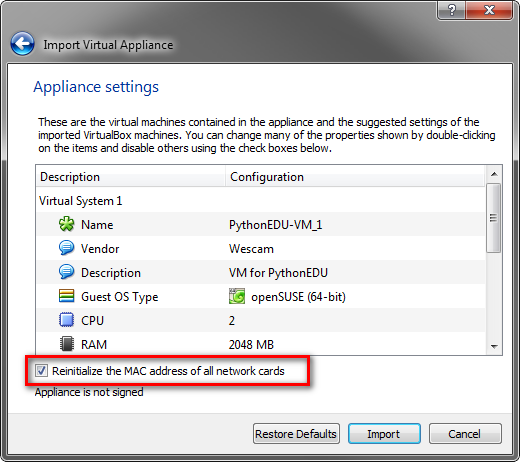
Fig. 1 Reinitializing the PythonEDU MAC IDs
- Click Import
The VM is large and will take time to import.
Start the VM by selecting it, then clicking the start button as shown in Fig. 2:
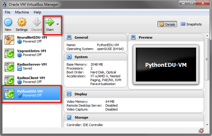
Fig. 2 Starting the PythonEDU VM
Using the Development Environment
The development environment is a VirtualBox virtual machine based on OpenSUSE Leap 42.3. When booted, you will be presented with the login screen as shown in Fig. 3:
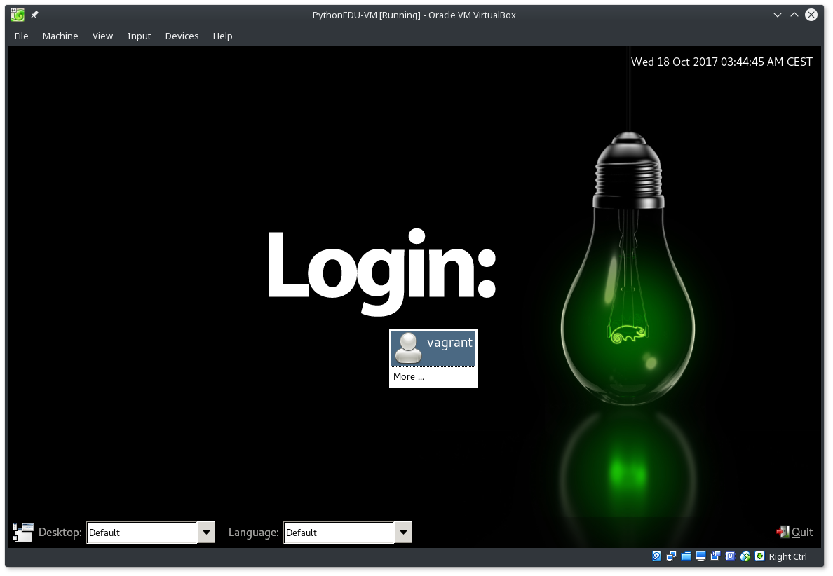
Fig. 3 Development Environment Login Screen
The credentials for logging in are:
| USER | PASSWORD |
|---|---|
| vagrant | vagrant |
| root | vagrant |
When you login, the desktop will look like that shown in Fig. 4:
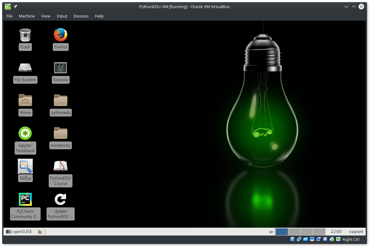
Fig. 4 Development Environment Desktop
This course makes heavy use of Firefox, Jupyter-Notebook and PyCharm. Take some time to get familiar with these tools and configure them to your personal preferences.
The Course Materials
The course materials are hosted on an external GIT repository and a linked clone is present on the VM. The material is in HTML format and can be read using any web browser. A link to the material is present on the desktop as shown in Fig. 5:
Fig. 5 Development Environment Course Materials Icon
Clicking on the icon shown in Fig. 6: will update the course materials in VM with what is in the external GIT repository. It will also rebuild the HTML files.
Fig. 6 Development Environment Course Materials Update Icon
The Jupyter-Notebook
To enforce the notion that you learn quickest when you put to use the thing you are learning, this course will make use of an interactive tool called Jupyter-Notebook. A quote from the Jupyter-Notebook website provides a quick overview of what it does:
“The notebook extends the console-based approach to interactive computing in a qualitatively new direction, providing a web-based application suitable for capturing the whole computation process: developing, documenting, and executing code, as well as communicating the result”
Using the Notebook app, you will be able to enter Python code in cells similar to what you would do in a Matlab program (in fact, many people use Jupyter-Notebook coupled with the NumPy and SciPy Python packages as a Matlab replacement). The output from Python as each cell is evaluated is provided after the cell. You can individually re-run any cell and refresh its output. You can add markdown around the cells to document what is going on. Finally, the notebook can be saved for use again at a later time.
Jupyter-Notebook can be started from the icon on the desktop as shown in Fig. 7:
Fig. 7 Development Environment Jupyter-Notebook Icon
Once started, a web-browser will be open which displays the Notebook dashboard as shown in Fig. 8:
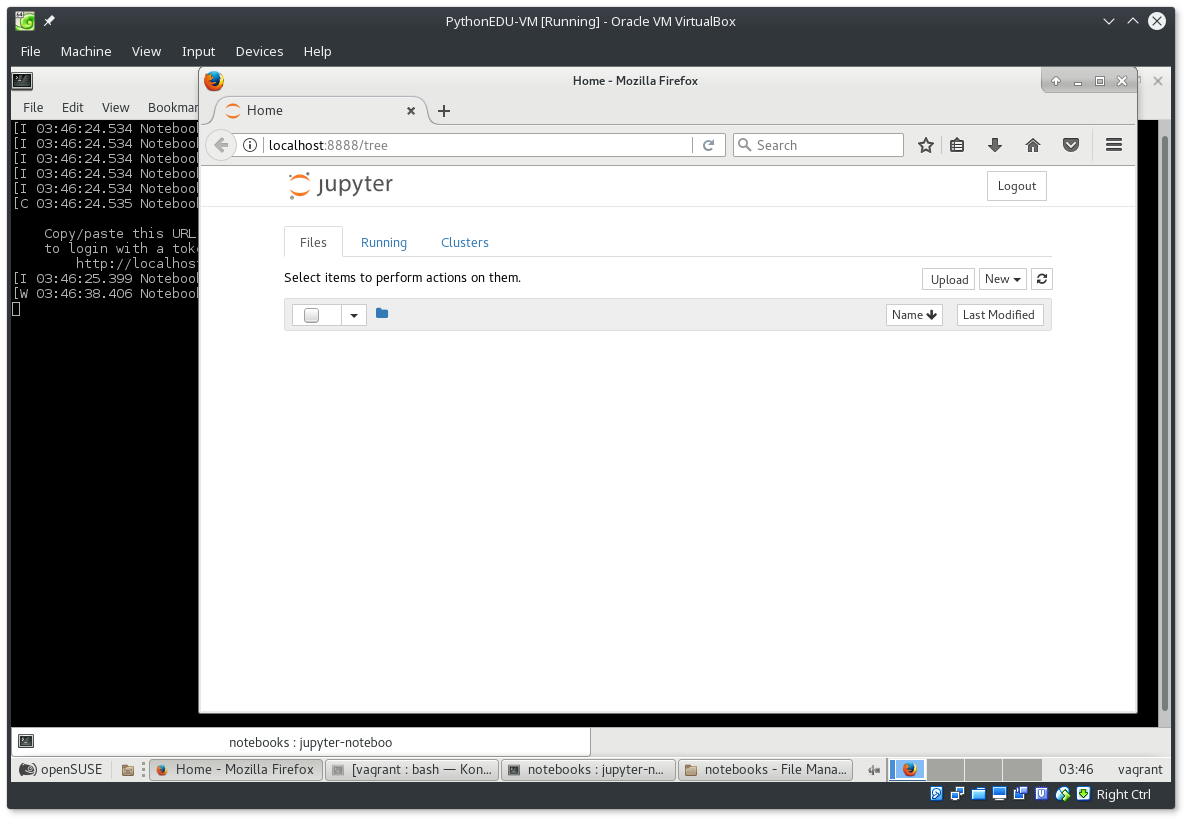
Fig. 8 Development Environment Jupyter-Notebook Dashboard
From the dashboard, click New -> Python3, to start a new notebook page using Python3 as the backend. After following these directions, you should wind up with what is shown in Fig. 9:
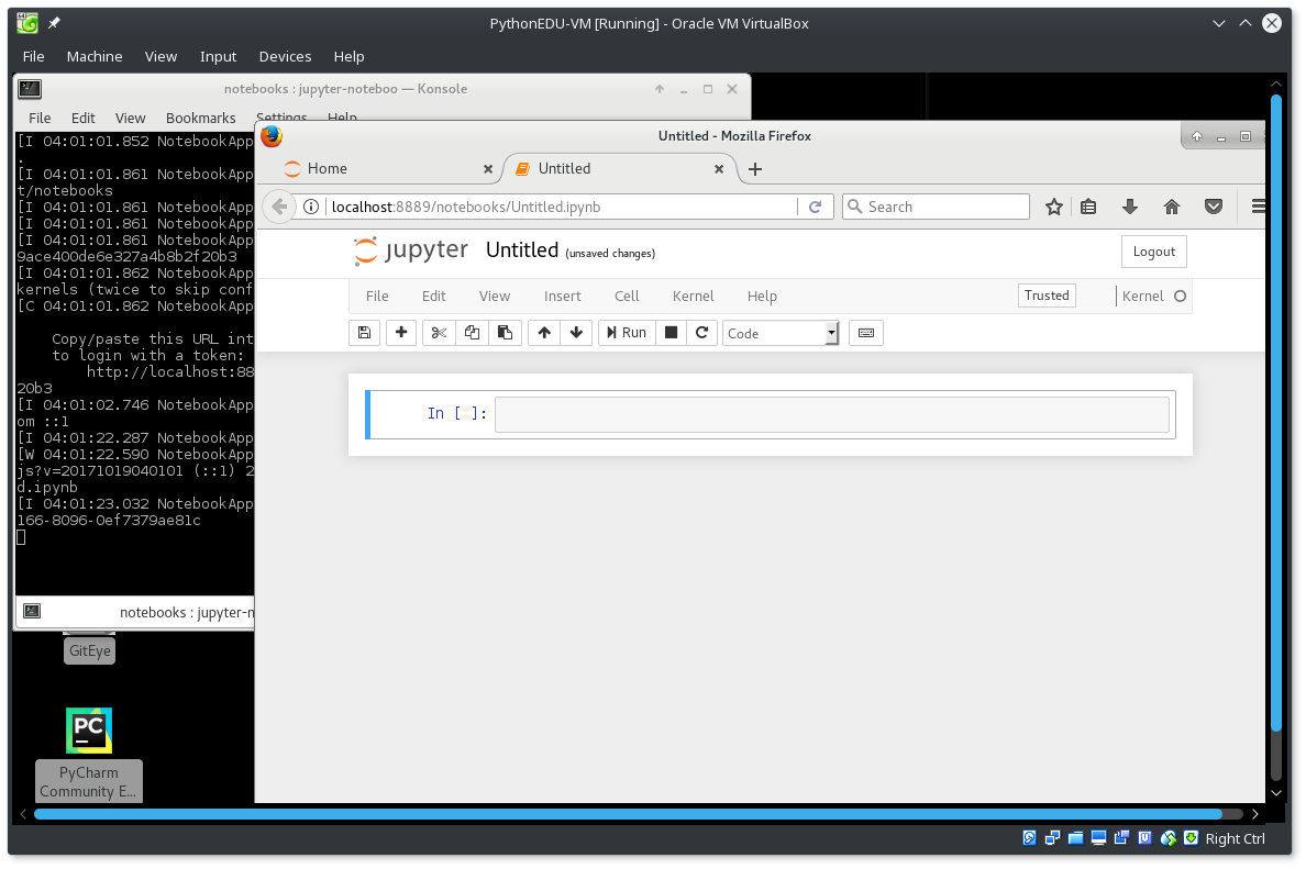
Fig. 9 Development Environment Jupyter-Notebook Empty Page
At this point, you can start entering Python code in the cells and executing them. You can enter multiple lines of Python in each cell; although, it’s generally more useful if you split up your commands across cells.
For example, enter, print("Hello World!"), in the cell. Then click run. Jupyter-Notebook will execute your code in a Python kernel running behind the scenes and then return the results to you below the code cell. You should wind up with what is shown in Fig. 10:
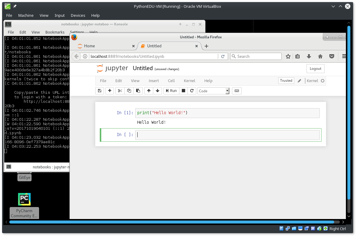
Fig. 10 Development Environment Jupyter-Notebook Hello World
When you are done your session and you close the browser tab, you will find a new notebook file in the dashboard as shown in Fig. 11:
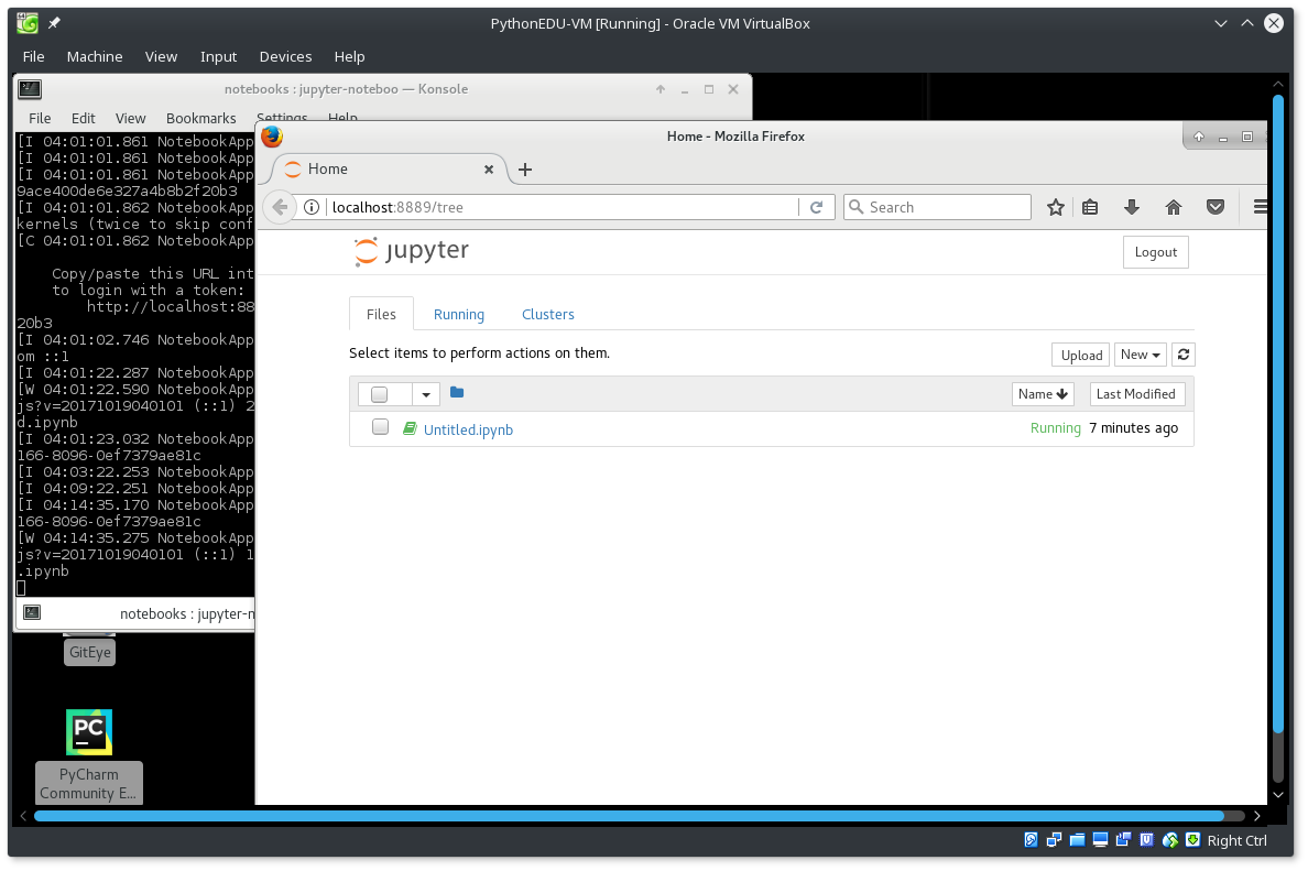
Fig. 11 Development Environment Jupyter-Notebook Saved Notebook
The file will have all the changes you have made to the notebook. You can come back and open the file at a later time and continue where you left off.
Note
It is possible to name the notebook from within it by changing it’s title.
This has been but the brief’est of brief overviews. To get a feel for how Jupyter-Notebook works and what you can do with it, please take some time to read the Jupyter-Notebook overview documentation before continuing with the course work.
Additionally, you can find a cheatsheet of Jupyter-Notebook commands here which should help you with learning the keyboard shortcuts.
Learning Layout
It can be useful to be able to try out code, in real time, while following the course material being presented. Jupyter-Notebook and the HTML documentation support this goal when both are open at the same time, similar to the arrangement shown in Fig. 12:
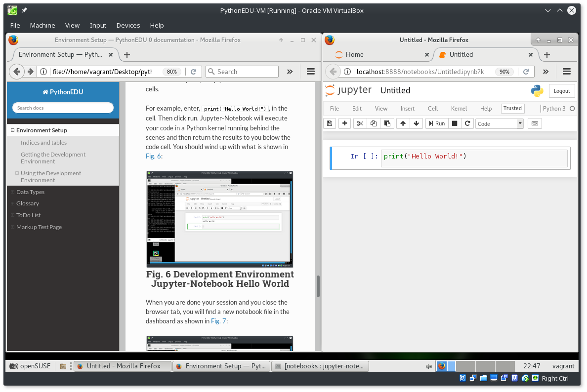
Fig. 12 Development Environment Learning Layout
PyCharm
As the Python programs being run grow larger and/or require debugging, it will be useful to develop your code using an IDE. Without trying to start any IDE wars that wind up with flaming arrows flying across the room, this section isn’t meant to condone one supreme IDE over all others. Instead, it is simply to introduce one IDE that is geared towards Python development, is free, and is pre-installed in the development environment. That IDE is called PyCharm (from JetBrains).
PyCharm can be started from the icon on the desktop as shown in Fig. 13:
Fig. 13 Development Environment PyCharm Icon
When PyCharm starts without a previous project to open (such as the first time you run it), it will present the welcome screen shown in Fig. 14:
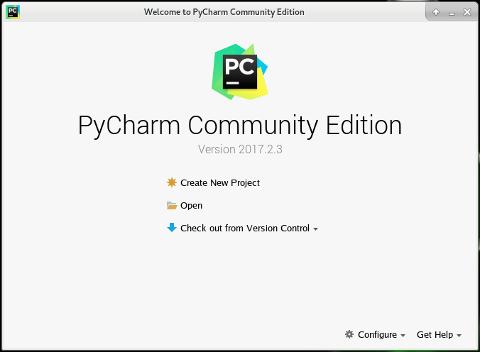
Fig. 14 Development Environment PyCharm Welcome Screen
If this is your first time running PyCharm, you should click on, Configure -> Settings, take a look around, and adjust things to your liking.
Some suggested items to adjust:
- Select a dark color scheme using, Appearance & Behavior -> Appearance -> UI Options -> Theme
- Show line numbers using, Editor -> General -> Appearance -> Show line numbers
It is not necessary to use all the sophistication that PyCharm offers. But, before you decide how you want to use it, you should take some time to get acquainted with it. The JetBrains website has material to get you up and running quickly:
One nice thing about PyCharm is if you like using it, it is cross-platform compatible so you can use it on Windows and OSX as well.
If you don’t like PyCharm, you are free to install and use your own. However, the instructors will be unable to assist you with issues related to IDEs other than PyCharm during the course.
Python Console
Prior to the existence of tools like Jupyter-Notebook and PyCharm, the classic way to interface to the Python interpreter is via a Python console. You may still find it useful to directly enter code into the console. There are 2 ways to get a Python console in the development environment:
- Open a shell console (the “konsole” icon on the desktop) and type ipython3.
- From within PyCharm, click Tools -> Python Console.
Note
The above instructions call the ipython3 interpreter which is a more powerful interactive shell then the stock python3 interpreter (think syntax highlighting, access to shell commands etc. but refer to here if you are curious). However, you are free to use the stock python3 interpreter if you wish.
When you start up the ipython3 console, you will get something like what is shown in Fig. 15. Notice it uses the Python prompt format, In [x]:.
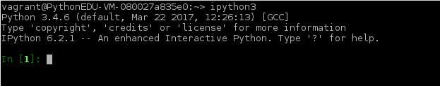
Fig. 15 Development Environment IPython Interpreter
When you start up the python3 console, you will get something like what is shown in Fig. 16. Notice it uses the prompt format, >>>. This is the classic Python prompt associated with the python interpreter.
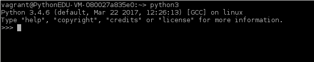
Fig. 16 Development Environment Python Interpreter
At the prompt, you can start entering python and the interpreter will go to work on it.
Note
For the remainder of the course, when you see the primary prompt, >>>, that will be an indication that something is being entered into the interpreter, regardless of which one it is that you are using.
Go ahead and try entering some code into the interpreter:
>>> print("Hello World")
Hello world
>>> for val in range(0, 5):
...    print(val)
...
0
1
2
3
4
Note
In the above console snippet, the ... is presented to the user when ever the console is waiting for additional input. It is called the secondary prompt.
When you are done with the interpreter, you can exit in 2 ways:
- Use
Control-d - Use the
exit()function
>>> exit()
Note
You must include the brackets when calling exit() as it is actually a Python function, defined by the interpreter implementation, that is being called.